
In today’s post, I will implement a matrix-based backpropagation algorithm with gradient descent in Python. For this purpose, we’ll only use the Numpy library to explain a bit of the mathematics behind the process (mainly multivariate calculus). To better cement the concept, we’ll build an XOR neural network (a network that learns to behave like an XOR logic gate).
Consider this post as part 2 of my series on neural networks, starting with “How to Build a Feedforward Neural Network in Python”.
Resources
If you are looking for a great resource on machine learning, I recommend the third edition of Aurélien Géron’s O’Reilly book: “Hands-On Machine Learning With Scikit-Learn, Keras & Tensorflow”.

The new edition came out in October of 2022 and has more up-to-date information on transformers and diffusion models. It also covers topics such as supervised and unsupervised learning, random forests, deep learning, natural language processing, and training and deploying Tensorflow models, among many more topics.
So, if you are interested, you can get it here using my referral link. The price is the same to you, but I might get a commission.
One other thing I like about the book is that it includes an end-to-end machine learning project to learn the entire pipeline of a data scientist.
XOR Neural Network
I mentioned that we’ll be using an XOR neural network as an example. It should make things easier to follow. Below you can find a graphical representation of this network.
An XOR logic gate takes two inputs and returns a single output. Here is the truth table for this gate:
| A | B | Output |
|---|---|---|
| 0 | 0 | 0 |
| 0 | 1 | 1 |
| 1 | 0 | 1 |
| 1 | 1 | 0 |
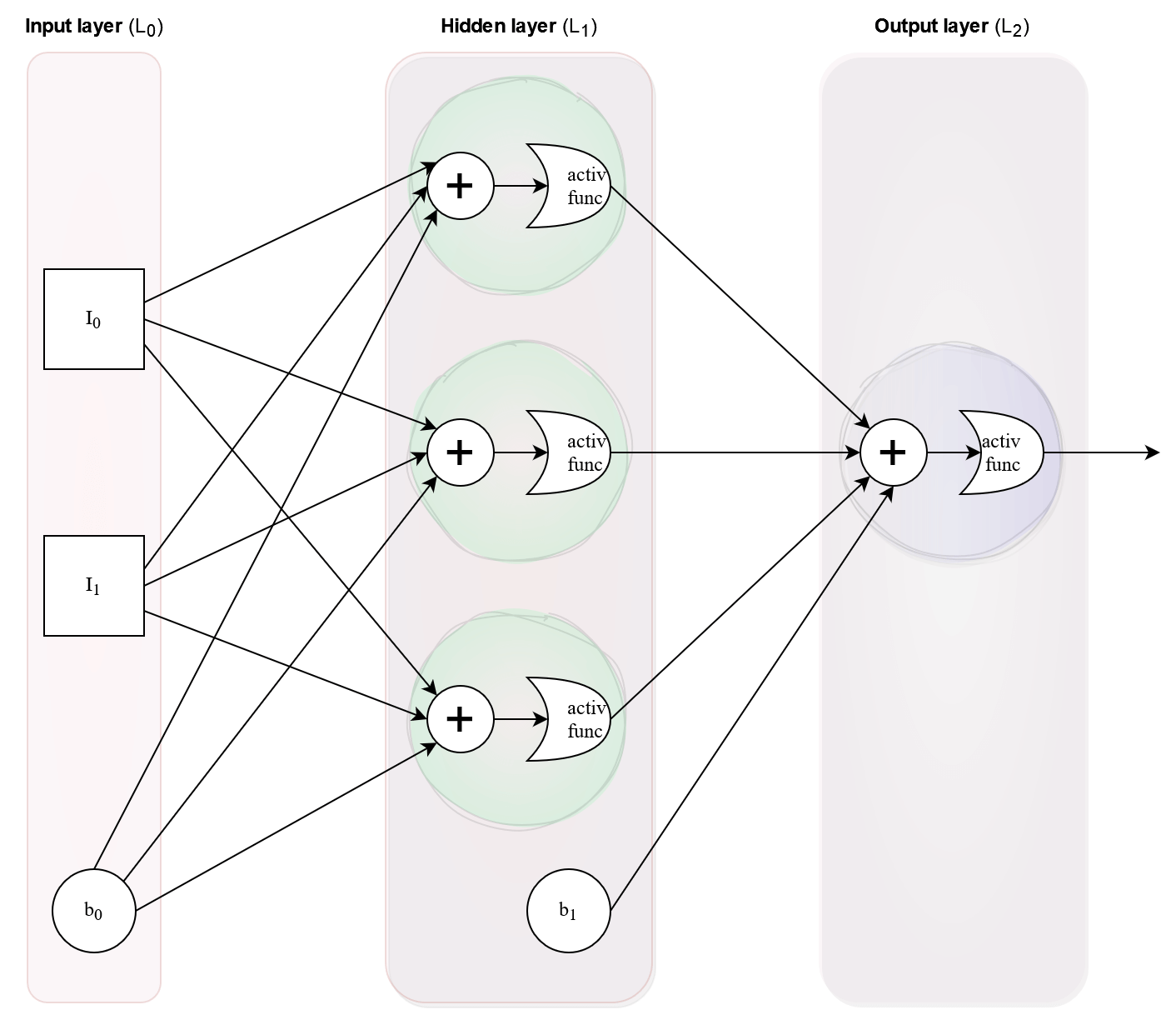
Therefore, we need a neural network with an input layer of two nodes and an output layer of one node. The hidden layer in between can technically be of any size, and there are different methods to decide on the best topology. For this example, we’ll just have three nodes in the hidden layer. Here is what the network looks like:

The Python code to create this network, using our NeuralNet class from the previous post is:
nnet = NeuralNet(topology=[2,3,1])
You can find the new jupyter notebook for this post here.
What Is Backpropagation?
First of all, remember that I’m not a mathematician, so terms and fundamental concepts might get fuzzy here. The goal of backpropagation is to figure out the error throughout the network during the training phase and update the network weights to reduce that error.
First, we perform a feedforward propagation of inputs, which is when the network gives us a prediction. Check my previous post on how to implement that part. With the prediction in hand, we can compare the result we got to the true value, or target, that we want the network to return.
To train a network, we need a way to correct the parameters (weights) based on their error, so we can fine-tune them. For a simple network like in our example, we have 2*3 + 3*1 = 9 total parameters to adjust or “train”. Actually, once we account for bias nodes and their weights, the total number of parameters will be 3*3 + 4*1 = 13. I will explain bias nodes in more detail below.
Backpropagation allows us to assign blame to each of the weights by using the method of gradient descent.
Gradient Descent
The concept of gradient descent is based on the “gradient” from multivariate calculus. The gradient is a vector of the partial derivatives of a function. Gradient descent is an optimization method where we try to find the local minima of a function.

In calculus, we find the slope of a function by taking its derivative. The slope is the direction of the highest ascent for the function. So, the gradient is basically the slope of a function in higher dimensions.
Since we are trying to minimize the error between what our network predicted and the real values, we need to travel in the opposite direction to the gradient.
By the way, with NumPy, if you have a vector A, you can flip its direction by changing its sign:
>>> import numpy as np

>>> A = np.array([-2,4.5,3])
>>> A
array([-2. ,  4.5,  3. ])

>>> -A
array([ 2. , -4.5, -3. ])
Differentiable Activation Functions
As I was saying above, gradient descent relies on taking the derivative of our activation function, so it makes it much easier when that function is differentiable. I talked about activation functions a bit more in my previous post. In this case, I will implement two custom functions that can return their own derivative.
Hyperbolic Tangent or Tanh

Fig. 2. shows the general shape of a tanh function centered at 0. The implementation in my notebook basically uses NumPy’s np.tanh method but adds the option to compute the derivative:
def tanh(x, derivative=False):
    if derivative:
        tanh_not_derivative = tanh(x)
        return 1.0 - tanh_not_derivative**2
    else:
        return np.tanh(x)
When derivative=False, this custom tanh uses Numpy’s np.tanh. However, when derivative=True, the function will return the derivative of tanh(x), which is simply 1 minus tanh(x) raised to the power of two:
\frac{d}{dx}\tanh(\vec{x}) = 1 - \tanh^2(\vec{x})ReLU Activation Function
A very popular activation function at this moment is the Rectified Linear Unit, or ReLU because of its computational simplicity. It is a composite function that returns 0 for any x <= 0 and returns x for any x > 0.

Numpy has a useful method, np.maximum to compare matrices element-wise against another matrix or scalar. We can use it to implement our vectorized ReLU function in Python:
def relu(x, derivative=False):
    if derivative:
        return 1 * (x > 0)  #returns 1 for any x > 0, and 0 otherwise

    return np.maximum(0, x)
When given an array and a scalar, np.maximum will compare each item in the array individually against the scalar, and return the bigger value.
The derivative for ReLU is easy to compute for the most part:
- It’s
0whenx < 0 - It’s
1whenx > 0
However, you may notice that ReLU is not differentiable when x = 0, so we need to handle that special case. We can either choose to give it a value of 0 or 1, and it seems the most common way is to assign 0 when x = 0 so that’s what I did here.
Here is an example using it:
>>> import numpy as np
>>> x = np.array([2, 4, 1, -0.3])

>>> x
array([ 2. ,  4. ,  1. , -0.3])

>>> relu(x)
array([2., 4., 1., 0.])

>>> relu([2, -1, 0.4, 0], derivative=True)
array([1, 0, 1, 0])
Adding Bias Nodes To The Neural Network
One important component of neural networks, which I omitted in my last post is the concept of a bias node.
In neural networks, bias nodes are positioned at each layer but they are not affected by the nodes in the previous layer. They always output 1 and have their own weights, which need to be updated during backpropagation. Here is another diagram showing our example neural network, including bias nodes.

Implementing Backpropagation in Python
To implement this algorithm, I repurposed some old code I wrote for a Python package called netbuilder and adapted it for this post. There are four main new functions in the NeuralNet class: _gradient_descent(), backprop(), train(), and _train_helper(). I also had to modify a few things in feedforward() and __init__() so that everything works smoothly.
As mentioned earlier, backpropagation works by taking the derivatives of the error function to compute the gradients. Since the error function depends on all the network’s layers, we need to apply the chain rule and get the derivatives of the activation functions in each layer, going from the last to the first. Take a look at this online resource if you want some more theory on the different stages of the calculations. Alternatively, take a look at the O’Reilly book on machine learning mentioned above for a hands-on implementation of different network types.
The basic steps for training the network are the following:
- Starting from the output layer and going backward:
- Compute the derivative of the error function
- Compute the derivative of the activation function for the final layer with respect to the layer inputs
- Compute the delta for this layer by multiplying the derivative of the error function with the derivative of the activation function
- Compute the gradient for the weight matrix by performing a dot product between the transpose of the inputs to the layer and the delta vector computed above.
- Apply gradient descent:
The change in weights is computed by the following equation:
\Delta{W_1} = -\alpha\nabla{W_1} + \mu\Delta{W_{1(t-1)}} Similarly, the update to the bias weight matrices is computed like this:
\begin{alignat*}
{2}\Delta{B_1} &= -\alpha\nabla{B_1}\ &+\ \mu\Delta{B_{1(t-1)}}\\ &= -\alpha\delta_1 &+\ \mu\Delta B_{1(t-1)}
\end{alignat*}
\begin{align*}
where:\\ \alpha &\rightarrow learning \ rate \\ \nabla W_1 &\rightarrow gradients\ for\ W_1\\ \mu &\rightarrow momentum \ factor \\ \Delta W_{1(t-1)} &\rightarrow change\ in\ weights\ from\ previous\ epoch \\ \Delta B_1 &\rightarrow change\ in\ bias\ weights \\ \Delta B_{1(t-1)} &\rightarrow change\ in\ bias\ weights\ from\ previous\ epoch\\ \delta &\rightarrow delta\ computed\ above
\end{align*}The term containing the momentum factor can be omitted.
- Now, with the change in weights, we can update the original weight matrix:
W_1 = W_1 + \Delta W_1
The equations described above are implemented in the function _gradient_descent(). Check it out to follow along.
The Backpropagation Code
class NeuralNet(...):
...
...
	def backprop(self, target, output, error_func,):
	    #Compute gradients and deltas
	    for i in range(self.size):
            back_index =self.size-1 -i                  # This will be used for the items to be accessed backwards

            if i == 0:   #final layer
                d_activ = self.output_activation(self.netIns[back_index], derivative=True)
                d_error = error_func(target,output,derivative=True)
                delta = d_error * d_activ
                #delta = np.multiply(d_error, d_activ)

                gradient_mat  = np.dot(self.netOuts[back_index].T , delta)
                bias_grad_mat = 1 * delta

                #-- Apply gradient descent
                self._gradient_descent(layer_idx=back_index, gradient_mat=gradient_mat, bias_gradient=bias_grad_mat)
The previous bullet points and the code above show how to compute the gradients for the output layer. For the rest of the layers, the process is not too different:
- Compute the derivative of the hidden activation function with respect to the layer inputs
- The derivative for the error in this layer will be given by the dot product between the delta vector from the previous layer (a higher layer since we are going backward) and the transpose of the weight matrix for this layer
- The new delta is the multiplication between the derivative of the activation function and the error computed above.
- Compute the gradient matrix similarly to the step described for the output layer
Here is that part of the code:
		...
		else:     #hidden layers
		    W_trans = self.weight_mats[back_index+1].T        #we use the transpose of the weights in the current layer
		    d_activ = self.hidden_activation(self.netIns[back_index],derivative=True)  #δl=((wl+1)Tδl+1)⊙σ′(zl)
		    d_error = np.dot(delta, W_trans)
		    delta = d_error * d_activ   #this should be the hadamard product,

		    gradient_mat = np.dot(self.netOuts[back_index].T , delta)
		    bias_grad_mat = 1 * delta

		    #-- Apply gradient descent
		    self._gradient_descent(layer_idx=back_index, gradient_mat=gradient_mat, bias_gradient=bias_grad_mat)
I separated the actual gradient descent code into its own function to keep the code easier to read. Here is _gradient_descent() and you can see how the equations above are implemented:
def _gradient_descent(self, layer_idx, gradient_mat, bias_gradient):

	#-- Calculate the changes in weights for all nodes and bias weights
	delta_weight =   (self.momentum * self.last_change[layer_idx])
							   - (self.learning_rate * gradient_mat[layer_idx])

	delta_bias_weights =  (self.momentum * self.last_bias_change[layer_idx]) \
	                    - (self.learning_rate * bias_gradient)

	#-- Update Weights
	self.weight_mats[layer_idx] += delta_weight    #the negative of the gradient is above
	self.bias_mats[layer_idx]   += delta_bias_weights

	#-- Keep track of latest delta weights for next iteration/epoch to compute momentum term
	self.last_change[layer_idx]      = 1 * delta_weight
	self.last_bias_change[layer_idx] = 1 * delta_bias_weights
Training the Network
The process to train the network is relatively simple once we have backpropagation implemented. It is just a matter of repeating the process over and over for a given number of iterations (epochs) or until the error is low enough. The full code can be found on the notebook companion for this post. I will just write the general pseudo-code here:
def train(epochs, inputs, targets, error_threshold, ...):
	for i in range(epochs):
		network_output = feedforward(inputs)
		error = error_function(targets, network_output)
		backpropagation(targets, network_output, error_function)

		if error <= error_threshold:
			break
The jupyter notebook includes training sets for other logic gates as well, but here is an example of network parameters that I tried for an XOR gate:
#-Network parameters
m           = 0.9            #momentum
a           = 0.01           #learning rate
init_method = 'xavier'       #weight initialization method
hidden_f    = tanh           #activation function for hidden layers
output_f    = tanh           #activation function for output layer
epochs      = 1000
batch_size  = 0
e_threshold = 1E-5           #error threshold to stop training

network_topology = [2, 3, 1] #shape of the network and its layers

input_data = np.array([[0,0],
                       [0,1],
                       [1,0],
                       [1,1]])

target_data = np.array([[0],
                        [1],
                        [1],
                        [0]])
Now we create and train the neural network using the parameters we defined above:
#-- create a new network for each set so they are independent of each other
nnet = NeuralNet(network_topology, hidden_activation_func=hidden_f, output_activation_func=output_f, init_method=init_method, momentum=m, learning_rate=a)
error = nnet.train(input_data, target_data, epochs=epochs, error_func=mean_squared_error, batch_size=batch_size, error_threshold=e_threshold)

# Test different inputs
print(f"\n\n{'='*40}\nTraining XOR gate:\n{'='*40}\n")

for i, sample in enumerate(input_data):
    output = nnet.feedforward(sample)
    sample_error = mean_squared_error(target_data[i:i+1], output)
    print(f"Testing Network:\n\tinput vector    : {sample}\n\toutput vector   : {output}\n\texpected output : {target_data[i]}")
    print(f"\tNetwork error   : {sample_error:.3e}\n")
and the output after 1000 epochs is:
========================================
Training XOR gate:
========================================

Testing Network:
	input vector    : [0 0]
	output vector   : [[0.00094011]]
	expected output : [0]
	Network error   : 4.419e-07

Testing Network:
	input vector    : [0 1]
	output vector   : [[0.96421877]]
	expected output : [1]
	Network error   : 6.401e-04

Testing Network:
	input vector    : [1 0]
	output vector   : [[0.98864499]]
	expected output : [1]
	Network error   : 6.447e-05

Testing Network:
	input vector    : [1 1]
	output vector   : [[0.00078335]]
	expected output : [0]
	Network error   : 3.068e-07
Wrapping Up
Try to run the example network in the notebook and see what you get. The results won’t always be as good as the ones I got here. If you are getting far-off outputs, maybe try running the training method again, or increasing the number of epochs. You could also experiment with changing the network topology.
Let me know what you thought of this post and if there are any issues you find.
You can also subscribe to my YouTube channel for videos on Python projects, automation, and crypto:
Finally, if you want to stay connected and up to date on what I post, you can join my newsletter here. I want this newsletter to be a useful resource of tips and tricks I learn and also a place to talk about new projects I might work on.