How To Build a Feedforward Neural Network In Python

Welcome back to another Python post. Today’s topic is about how to create a feedforward neural network in Python, from scratch. That means, without using Tensorflow, Keras, Pytorch, etc. The main library we’ll be using is numpy, which is the computing library for Python.

I usually like to understand the underlying concepts of how things work, before I use a tool like Tensorflow to handle things for me. Doing it myself allows me to better learn the concepts and to have a stronger foundation for implementation. In particular, I would like to cover some of the linear algebra concepts that underpin the workings of deep neural networks.

There are many types of artificial neural networks: convolutional, fully connected, recurrent, etc. This post is specifically about fully connected, feedforward networks and how they work. To learn about implementing backpropagation from scratch, read my next post in the series.

Resources

If you are looking for a great resource on machine learning, I recommend the third edition of Aurélien Géron’s O’Reilly book: “Hands-On Machine Learning With Scikit-Learn, Keras & Tensorflow”.

The new edition came out in October of 2022 and has more up-to-date information on transformers and diffusion models. It also covers topics such as supervised and unsupervised learning, random forests, deep learning, natural language processing, and training and deploying Tensorflow models, among many more topics.

So, if you are interested, you can get it here using my referral link. The price is the same to you, but I might get a commission.

One other thing I like about the book is that it includes an end-to-end machine learning project to learn the entire pipeline of a data scientist.

What Are Neural Networks?

Artificial neural networks try to mimic the way the human brain works. There are “neurons” that perform simple computations by themselves. However, by stacking together layers of these “neurons”, a neural network can exhibit complex and emergent behavior.

Of course, the human brain is much more complicated than that, but the analogy makes it simple to understand.

Mathematically, artificial neural networks are functions that take an input and produce an output. They are called “universal function approximators” functions because with appropriate weights and training, they can approximate the behavior of a wide range of functions.

Neural Networks As Matrices

Once we have the basic concept of artificial neural networks, we need to find a way to represent them in code. For me, the most natural way to do this is by using matrices from linear algebra.

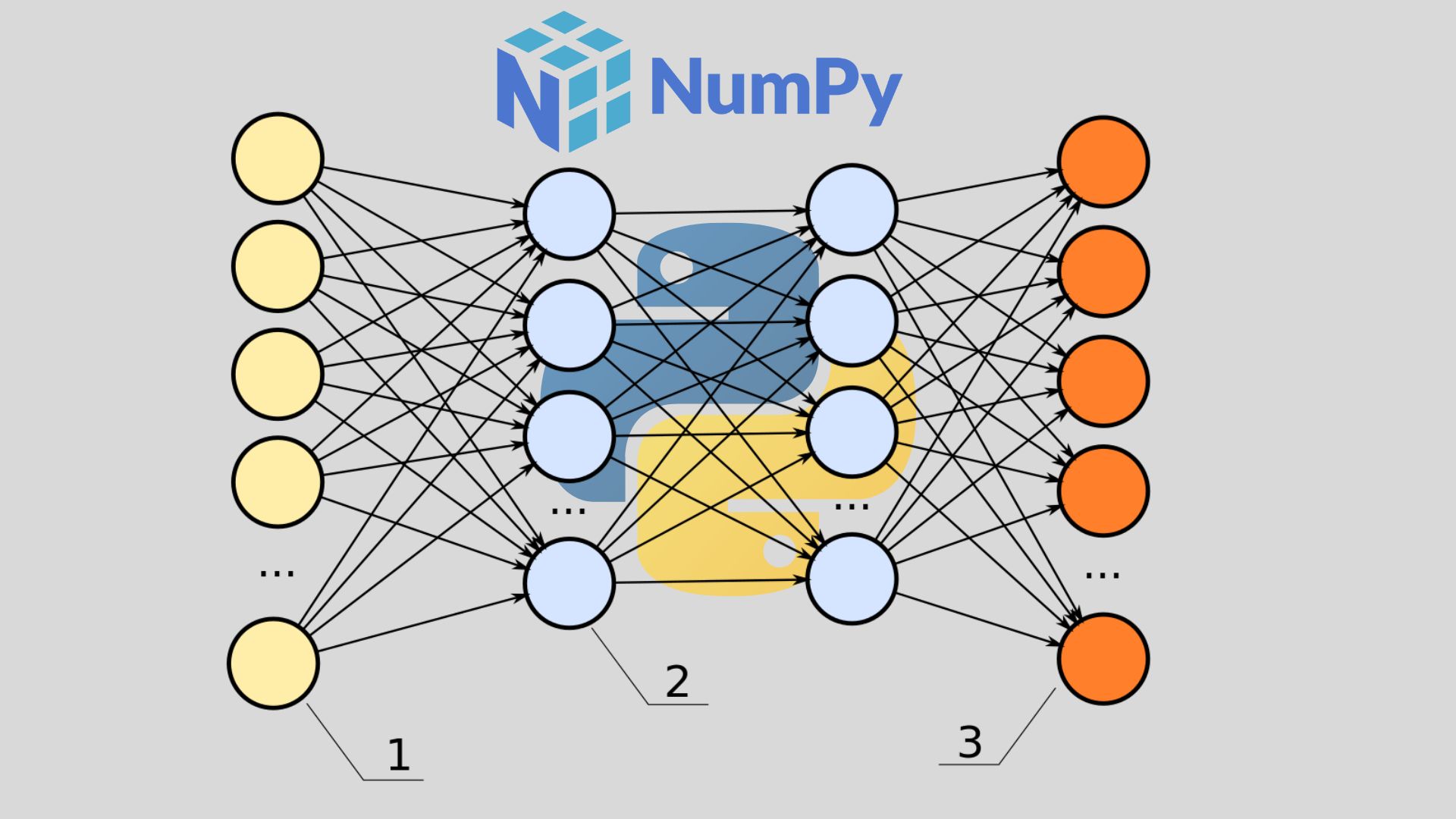
Let’s use this network as an example. Here we have 3 layers in total. There is the input layer with 3 nodes, then one hidden layer with 4 nodes. Finally, we have the output layer, with 2 nodes or neurons.

In a fully connected feedforward neural network, each neuron in a layer has a connection to all the neurons in the next layer. Additionally, each connection has a weight (a number) associated with it. This number is usually set at random at the beginning and then it is fine-tuned during the training (learning) phase.

We can represent this network as a series of matrices, where each row represents a node, and each column is the connection to the next layer’s nodes.

For instance, in the example network in the image, we will have 2 matrices in total. The first matrix represents the connections between the input layer and the hidden layer, resulting in a 3×4 matrix.

We have 3 rows, one for each input node, and the values along that row are all the connections from that input node to all the hidden nodes in the next layer. We do the same for the next two layers (L2 and L3), resulting in a 4×2 matrix.

Neural Network In Python

In Python, we could represent the network as a class, and if you need a refresher on Python classes, check out my previous post. Here is a simple implementation:

import numpy as np


class NeuralNet(object):
    RNG = np.random.default_rng()


    def __init__(self, topology:list[int] = []):
        self.topology    = topology
        self.weight_mats = []

        self._init_matrices()


    def _init_matrices(self):
        #-- set up matrices
        if len(self.topology) > 1:
            j = 1
            for i in range(len(self.topology)-1):
                num_rows = self.topology[i]
                num_cols = self.topology[j]

                mat = self.RNG.random(size=(num_rows, num_cols))
                self.weight_mats.append(mat)

                j += 1

We created a NeuralNet class that contains the connection weights as numpy arrays (matrices).

The class initializer also takes a parameter topology, that tells the constructor what the shape of the network will be. This parameter takes a list of integers, each one representing the number of neurons per layer that we wish the network to have.

For our example image, we would pass the following values: topology=[3, 4, 2] because we have 3 input nodes, 4 nodes in the hidden layer, and 2 in the output layer. Each item in topology represents another layer.

This also allows us to make a network as deep as we want. For example, topology=[3, 10, 10, 10, 20, 10, 10, 5] would result in a network with 8 layers (6 hidden plus the input and outputs).

The matrices are initialized to random values. I did not pay much attention to the initialization method because it is not the focus of the post. However, it can have a big effect on training times if weights are not initialized with some care. I will cover this topic in a later post.

Feed-Forward Propagation

A neural network “thinks” when we feed it some input and we let the information flow throw the layers until it reaches the output layer. This flow is the feed-forward propagation, and it involves some simple linear algebra, specifically, matrix multiplication and the dot product.

Matrix Multiplication and Dot Product

One thing to keep in mind when performing matrix multiplications is that the inner sides of both matrices need to be the same size. This requirement exists because of the dot product (explained further down). Here is what I mean by that:

Suppose we have two matrices: matrix A, and matrix B.

Matrix A is 4×3 (4 rows and 3 columns), while matrix B is 3×5 (3 rows and 5 columns). We can do this multiplication because the inside size of both matrices is 3.

The result of this multiplication will be a new matrix T with dimensions 4×5 (the outside dimensions of the initial matrices). In general, if you have a matrix of size NxG and another of size GxM, you can multiply them, and their result will be a matrix of size NxM.

Then, the actual multiplication process involves repeated dot product operations. Numpy has a function for this, but we will cover it briefly.

For the dot product, you need two vectors (1-dimensional arrays), one from each matrix. We start by taking the first row of matrix A and the first column of matrix B.

Then, we multiply each of their elements and add them together into a single number.

The dot product above will produce the first element in the resulting matrix T, or element t₀₀.

Matrix Multiplication With NumPy

Here is an example of how to perform a matrix multiplication between two 2-D matrices with the numpy.dot method:

>>> import numpy as np  

>>> A = np.random.rand(3,4)
>>> A
array([[0.58117773, 0.4367495 , 0.17583791, 0.97634689],
       [0.81055793, 0.84320293, 0.32176276, 0.05177668],
       [0.57115715, 0.44588042, 0.07577211, 0.7077594 ]])

>>> B = np.random.rand(4,5)
>>> B
array([[0.41545468, 0.60417725, 0.37690862, 0.18888787, 0.51163858],
       [0.03382709, 0.01476612, 0.90917151, 0.8484174 , 0.84380944],
       [0.67937006, 0.23757462, 0.23856111, 0.06583954, 0.56261105],
       [0.51240073, 0.83905954, 0.29712731, 0.68606154, 0.05471066]])

>>> T = np.dot(A, B)
>>> T.shape
(3, 5)
>>> T
array([[0.87596684, 1.21857125, 0.94817851, 1.16173444, 0.81823123],
       [0.61039958, 0.62205787, 1.16426669, 0.9251993 , 1.31007532],
       [0.66650649, 0.96351789, 0.84902675, 0.97673267, 0.74981635]])

Feeding Input To the Neural Network

Our example network has 3 input nodes. That means we need to provide it with an input vector (or matrix) of size 1×3. Since our first weight matrix is of size 3×4, the first matrix multiplication will look like this:

the result of the matrix multiplication will be a new vector of 4 elements. In matrix notation, we could say that it has a size of 1×4, which is perfect since the next layer’s matrix is of size 4×2 and the size condition is satisfied.

However, before we multiply this new vector by the next matrix, we need to transform it a little bit. This transformation is done by using an activation function, and that’s what we’ll be looking at next.

What Is An Activation Function?

The concept of an activation function comes from the human neural network analogy. In real life, neurons have an activation potential. If the input that reaches a neuron is not strong enough, then the neuron will not fire and information will not flow to the next layer.

In the case of artificial neural networks, activation functions can add non-linearity to the network. I think this post explains well why activation functions are important.

In any case, each neuron in the network has an activation function, and it applies this function to the input it receives. Because we are using numpy, we can take advantage of vectorization and apply all activation functions for a layer at the same time.

Types of Activation Functions

There are different activation functions that can be used. Some common ones are sigmoid functions, which have the convenient characteristic of being easily differentiable (taking their derivative is computationally easy).

In the last example, after performing the first matrix multiplication, we are left with a new vector \vec{I_{(1x4)}}. It is at this stage that we apply an activation function on this vector, element-wise. One common function for this is the hyperbolic tangent (tanh) function. The tanh function is a type of sigmoidal function, and its derivative is easy to compute, so it is the one we’ll be using for this example. It also maps any value to a range of [-1,1].

Some activation functions you might hear about are the following:

• Rectified Linear Unit (ReLU)
• Leaky ReLU
• Sigmoidal functions
• Hyperbolic Tangent (tanh)
• Softmax

You should analyze which ones are the most convenient for the approach you are trying to take.

Feedforward Propagation In Python

Here is the code that I will be using to implement feedforward propagation with Python. The new method is part of the NeuralNet class we created above.

class NeuralNet(object):
    ...

    def feedforward(self, input_vector):
        I = input_vector
        
        for idx, W in enumerate(self.weight_mats):
            
            I = np.dot(I, W)
            
            if idx == len(self.weight_mats) - 1:
                out_vector = np.tanh(I)  #output layer
            else:
                I          = np.tanh(I)  #hidden layers
            
        return out_vector

In this code, I’m using tanh as the activation function for all the layers. However, we can actually use a different activation function for the hidden layers than the output layer. For instance, if the network is learning to predict probabilities, then maybe the sigmoid function will be better because it outputs a value between [0,1], instead of [-1,1] like tanh.

Now we can create an instance of our NeuralNet class and call the feedforward network.

First, I passed topology=[3,4,2] to match the example network we’ve been using. Then I’m calling the feedforward method with some random values. These values are in a list, which numpy will automatically convert into a numpy array before computing the dot product for us. Just remember that the input needs to be the same size as the network’s input layer.

Considerations And Caveats

The focus of this post was to show how feedforward propagation happens in the background. Some things that I omitted completely here are:

• Proper network weight initialization
• Bias nodes
• Pre-processing input before forward propagation
• Training the network using backpropagation

If you want to see a backpropagation implementation, read my next post in the series.

Final Thoughts

We have seen that the feedforward process for a neural network is basically a series of matrix multiplications, with activation functions in between. Most of it is linear algebra, and numpy allows us to create this functionality on our own.

I find it easier to comprehend these kinds of concepts after doing them by hand first, and I think that many other people are going to feel the same way. Finally, here is the repository where I’ll be adding code related to neural networks, including the one in this post.

If you want to hear about the next posts in this neural network series, consider joining the newsletter mailing list.

Also, if you have any questions, or if I made a mistake, let me know in the comments.